3  How these systems work: from the eGFR on a chemistry panel to the next word

AIM-1 · AIM-2 · about 75 minutes

NoteWhat you’ll learn

By the end of this chapter you will be able to:

1. Explain, using eGFR as the worked example, what it means for a formula to be learned from data rather than worked out from theory, and name its predictors, its response, and the population it was learned from.
2. Tell supervised from unsupervised learning by asking what the training data contains, and classification from regression by asking what kind of answer the model gives.
3. Say why a model’s performance on data it has already seen tells you nothing useful, and why separate training and test data is the least you should accept.
4. Describe in plain words what a language model computes at each step, and use that description to explain a made-up citation or a confident wrong answer as a natural result of how the model works, not as a bug.
5. Name two built-in limits of the context window: it is a shared budget, and material buried in the middle gets less reliable attention. Say what each one changes about how you will prompt.

Time. About 22 minutes of reading, 27 minutes of watching, 20 minutes of doing, and 6 minutes for the check and the closing question. No math and no coding are assumed. The only equation in the chapter is one you already use. You need a browser and your institutional ChatGPT Edu or Microsoft Copilot account, or whatever assistant your school provides. Nothing installs, and nothing asks you for a phone number.

3.1 The number nobody measured

Pre-operative clinic, your surgery sub-internship. A 62-year-old woman is being worked up for a laparoscopic cholecystectomy. Her basic metabolic panel is back, and one line is flagged.

Basic metabolic panel · collected 07:12

Sodium	139		136–145 mmol/L
Potassium	4.1		3.5–5.1 mmol/L
Creatinine	1.10		0.50–1.10 mg/dL
eGFR (CKD-EPI 2021)	57	L	>60 mL/min/1.73 m²

Illustrative panel, made up for this chapter; not a real patient’s result.

The attending asks whether her kidneys are all right for the contrast CT the surgeon wants. You answer the way everyone answers: “eGFR 57, stage 3a, mildly reduced, probably fine with hydration.” The attending nods. That is the whole conversation. You will have it several hundred times in intern year.

Now the question at the center of this chapter. Nobody measured her glomerular filtration rate. Measuring it means infusing a marker that the kidney filters and does nothing else with, such as inulin or iohexol, and timing how fast it clears. That takes hours, and it is done almost only in research studies. The 57 on the panel was computed from three things the lab did have: her creatinine, her age, and her sex. Something turned those three numbers into a kidney function. You trusted it enough to clear her for contrast.

Where did that formula come from? Not from physiology. Nobody worked it out from the physiology of nephrons. It was learned from data. A few thousand people did have their GFR measured. Their creatinine, age, and sex were fed to a computer with one instruction: find the formula that best predicts the measured number. The eGFR is a model. It is the model you already trust most, and you have never once asked what it was trained on.

Remember this patient. She weighs 45 kilograms and has lost a good deal of muscle over a year of on-and-off illness. We will come back to her.

3.2 Why this matters

In three months you will meet a dozen of these. A sepsis alert that fires in the EHR. A risk score that decides who gets a phone call after discharge. A scribe that drafts your note. A chatbot that answers a dosing question at 2 a.m. Every one of them is the same kind of object as the eGFR: a formula learned from some population, applied to your patient, with failures that follow from how it was built. This chapter does not teach you to build these things. It teaches you to look at one and predict how it will fail, in the thirty seconds before you act on it.

The second half of the chapter does this for the language model in particular, because its failures are the strangest and the smoothest. It will give you a citation that does not exist, formatted perfectly. It will do so for a reason that follows directly from what it computes. Once you can say that reason out loud, “it hallucinates” stops being an empty phrase. It becomes a prediction about when to check.

3.3 How it works

3.3.1 A formula learned from data

The eGFR your lab reports almost certainly uses the CKD-EPI 2021 equation. Here is how it was made. Researchers combined ten studies in which 8,254 people had their GFR measured directly with a filtration marker. Each person also had a creatinine measured by a standard method, an age, and a sex on record. The researchers then fit an equation that predicts the measured GFR from those three inputs as closely as possible across all 8,254 people. “Fit” means a computer tried numbers in the equation until the predictions were as close to the measured values as they could get. They then tested the equation on a separate set of 4,050 people from twelve other studies, whose measured GFR the equation had never seen (Inker et al., 2021).

That paragraph contains every term you need for the rest of the course. Here they are, named:

• Predictors are the inputs: creatinine, age, sex. The literature also calls them features or variables.
• The response is the thing being predicted: measured GFR. Also called the label, the outcome, or the truth.
• The training set is the 8,254 people whose predictors and response were used to fit the equation. The test set is the 4,050 people the equation was checked on afterwards.
• The model is the equation itself, once fit: eGFR = f(creatinine, age, sex). The f is whatever shape the fitting settled on. For CKD-EPI it is a handful of exponents and multipliers. For the systems later in this chapter it is billions of numbers. The role is the same.

Figure 3.1 shows what that model connects. The thing you want to know is on the right. The thing the lab can measure is on the left. The equation is the bridge, and the bridge was built from a specific set of people.

A stand-in like this, something you measure because the real thing cannot be measured, is called a proxy. The first of the course’s three recurring lessons is proxies fail: the stand-in and the real thing can come apart, and they come apart for some patients more than for others. The bias and equity chapter depends on that lesson. This chapter’s job is narrower: to show you the bridge at all.

flowchart LR
  accTitle: What the eGFR equation takes in and what it stands for
  accDescr: Flowchart. Three inputs the lab has, serum creatinine, age, and sex, feed an equation learned from 8,254 people with measured GFR, which outputs the eGFR on the panel. A dotted arrow shows the eGFR standing in for measured GFR, which is never done in routine care. A grey box, muscle mass, diet, and drugs that block secretion, feeds creatinine without touching measured GFR.
  subgraph IN["What the lab has"]
    direction TB
    cr[Serum creatinine]
    age[Age]
    sex[Sex]
  end
  eq["eGFR = f(creatinine, age, sex)<br/>learned from 8,254 people<br/>whose GFR was measured"]
  out["eGFR<br/>(a number on your panel)"]
  truth["Measured GFR<br/>(iohexol or iothalamate clearance;<br/>never done in routine care)"]
  cr --> eq
  age --> eq
  sex --> eq
  eq --> out
  out -. "stands in for" .-> truth
  muscle["Muscle mass · diet ·<br/>drugs that block secretion"]:::grey -.-> cr
  classDef grey fill:#eee,stroke:#999,color:#555

Figure 3.1: What the eGFR equation takes in and what it stands for. The equation was learned from 8,254 people with measured GFR. It is a bridge from what a lab can measure to what a clinician wants to know. Anything that changes creatinine without changing GFR (grey) crosses the bridge unnoticed. Redrawn from the description of the CKD-EPI 2021 development in Inker et al. (2021).

Three things follow from “learned from data”. Each one is a question you can ask of any model.

The truth column existed. For every one of the 8,254 people, someone had actually measured the real GFR. That is what makes this supervised learning: the training data contains the answer, and the model learns to reproduce it. Unsupervised learning is what you do when there is no answer column, only patterns to find. Sorting 10,000 tumor expression profiles into groups, without being told which are which, is unsupervised. The test is simple: does the training data contain the thing you want predicted?

The model gives a number. eGFR is a quantity, so this is regression: the output is a value on a scale. If the same inputs were used to output “CKD: yes or no”, that would be classification: the output is a category. Most clinical prediction tools are one or the other, and the difference decides how you judge them. A regression is wrong by an amount. A classification is wrong by a kind, a miss or a false alarm, and those two kinds cost different people different things.

The model is exactly as good as the people it was fit to. The 8,254 were mostly participants in kidney research studies. 31.5 percent of them were Black. None were children. None were your patient. For anyone outside that set, the equation is guessing beyond what it saw. Statisticians call that guess an extrapolation. The history of the equation is a history of finding out where the guess failed.

3.3.2 The history of one equation is the history of its training set

Table 3.1: Three generations of the eGFR equation, rebuilt from the numbers in the papers. Each one is a formula learned from a population, and each one’s known failure is in people outside that population.

Equation	Year	Learned from	Tested on	What broke, and where
MDRD	1999	1,628 patients with chronic kidney disease, of whom 1,070 were the training sample	The remaining 558	Fit to people with reduced GFR; gave values that were too low at higher GFR, so healthy people were labeled as diseased (Levey et al., 1999; Levey et al., 2009)
CKD-EPI	2009	8,254 participants in 10 studies	3,896 in 16 studies	More accurate at higher GFR, but included a term that adjusted the result for Black race; the 2021 study showed that term overestimated measured GFR in Black adults by a median of 3.7 mL/min/1.73 m² (Inker et al., 2021; Levey et al., 2009)
CKD-EPI 2021	2021	8,254 participants in 10 studies, refit without race	4,050 in 12 studies	Now recommended for all US laboratories; the refit without race still gives values a few mL/min too low in Black adults and a few mL/min too high in non-Black adults, and a cystatin C version is more accurate (Delgado et al., 2021; Inker et al., 2021)

Read the last column as a pattern, not as nephrology. Every row says the same thing: the model was fit to these people, and here is what happened to those people. the bias and equity chapter takes up why the race term was there in the first place and who was harmed by it. For this chapter the point is narrower, and it applies to every model. The training population is a property of the model, as much as the equation is. You cannot judge the one without knowing the other.

3.3.3 The loop, in general

Every model in this course, from the eGFR to the chatbot, was built by the same loop. Figure 3.2 draws it once.

flowchart LR
  accTitle: The loop every learned model comes from
  accDescr: Flowchart. Raw material such as labs, images, notes, or text becomes predictors. The truth for each case, such as measured GFR, sepsis yes or no, or the next word, joins them in a learning step that finds a function f so that truth is approximately f of predictors. The result is a model, and a new case with unknown truth goes through the model to produce a prediction.
  raw[Raw material:<br/>labs, images, notes, text] --> pred[Predictors]
  truth[Truth for each case:<br/>measured GFR, sepsis yes/no,<br/>the next word] --> learn
  pred --> learn["Learn: find f so that<br/>truth ≈ f(predictors)"]
  learn --> model["Model: response = f(predictors)"]
  new[New case, truth unknown] --> model --> ans[Prediction]

Figure 3.2: The loop every learned model comes from. Turn the raw material into predictors, collect the truth for each case, learn a function that predicts truth from predictors, then apply it to a case whose truth you do not have. The eGFR, a sepsis alert, and a language model differ only in what fills the boxes.

You now have two questions that sort any model in about ten seconds. They are the ones the Check asks you to apply:

Table 3.2: Two questions that sort any model.

Question	If yes	If no
Does the training data contain the answer?	Supervised	Unsupervised
Does the model give a category?	Classification	Regression (a number)

3.3.4 Why performance on data it has seen tells you nothing

Here is the mistake the eGFR researchers avoided, and the one every vendor slide invites you to make. Suppose you fit a formula to 8,254 people. Then you report how well it predicts GFR in those same 8,254 people. You have measured how well the formula memorized them, not how well it will work on the next patient. A flexible enough model can fit its training data perfectly and be useless. Its performance on data it has already seen is not evidence. It is a description of the fitting.

Figure 3.3: Every one of these fits the same data. The one on the bottom right passes through every point, and it is the worst model of the twelve. xkcd 2048, Curve-Fitting, by Randall Munroe, CC BY-NC 2.5 (non-commercial use only).

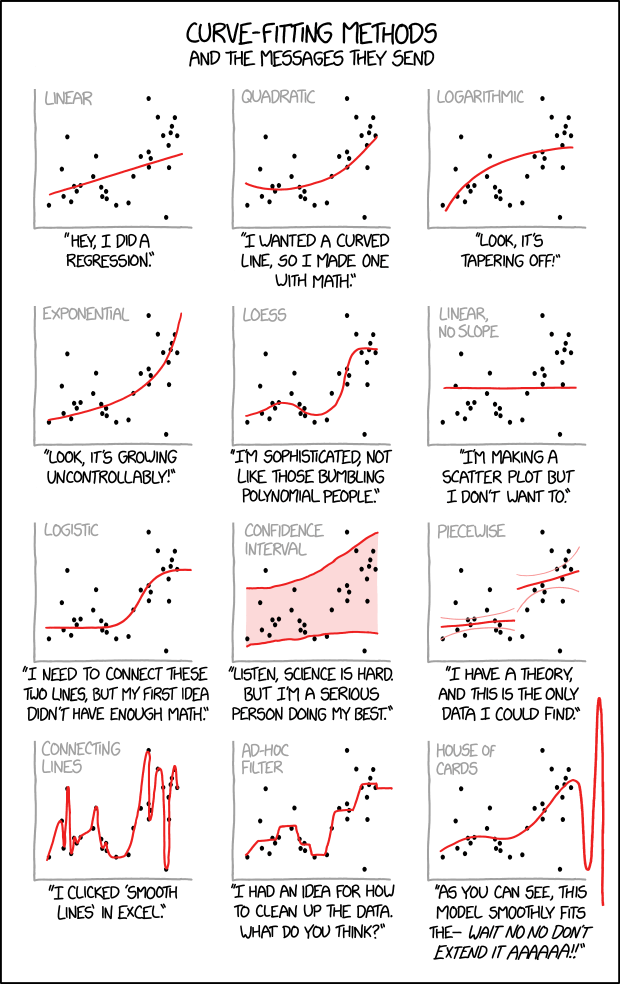
That is why separate training and test sets are the least you should accept. You fit on one set of cases. You report performance on a different set the model never saw. The 4,050-person validation set in the eGFR paper is that second set. When a claim about a model gives you one number and does not say which set it came from, you do not yet have a number.

There are two ways to get this wrong, and each has a name. A model that is too simple cannot capture the real relationship no matter how much data it sees: the straight line through a curve. Statisticians call that error bias, in a technical sense that has nothing to do with the social meaning. A model that is too flexible learns the random scatter in its particular training set along with the real pattern. It fits those cases very closely and the next case badly: the wiggle through every point. That error is variance. You will see both in the exercise, in about eight minutes, on your own screen. The third sentence you write there is the one you will apply to every performance claim you are ever shown.

The clinical version of the same failure is dataset shift: the patients the model meets in real use differ from the patients in its training set, so performance measured during development does not hold (Finlayson et al., 2021). Here is an example. One EHR vendor built a sepsis model that runs in hundreds of US hospitals. One academic center tested it on its own 38,455 hospitalizations, a test the literature calls external validation, because the testers had no part in building the model. The model had an area under the curve of 0.63, on a scale where 0.5 is no better than chance and 1.0 is perfect. It missed 67 percent of patients with sepsis, and it alerted on 18 percent of all admissions (Wong et al., 2021). Nobody had lied about the development performance. It simply had not been measured on patients like those.

ImportantThe one sentence

A model’s performance on the population it was built from is the optimistic number. That is the third of the course’s three recurring lessons, the published number is the optimistic one, in its first form. Ask what it was trained on, and ask what it was tested on. If those are the same set, you have learned nothing yet.

3.3.5 From tables to words

Everything so far had a table: one row per patient, one column per predictor, one column of truth. A language model is the same loop with a different table. Seeing that is the key point.

Take any sentence from the internet: the patient was started on empiric. Split it into tokens, which are words or pieces of words. “Empiric” might be one token and “vancomycin” three. Now the predictors are the tokens so far, and the truth is the very next token. You do not need anyone to label anything, because the next word is already in the text. Every sentence ever written becomes a training case, with no labeling work. That is why these models could be trained on a very large fraction of the written internet.

To make tokens usable by the loop, each one is turned into a list of numbers, called an embedding. The numbers are chosen so that tokens used in similar contexts get similar numbers. “Vancomycin” ends up near “linezolid” and far from “Tuesday”. That is the “raw material to predictors” box of Figure 3.2, done for words.

The model is then trained to do one thing: given the tokens so far, produce a probability for every possible next token. Then one token is picked, at random but weighted by those probabilities. It is added to the end, and the process runs again. A paragraph of smooth medical prose is a few hundred repetitions of predict the next token, pick one, repeat. Your phone’s keyboard does this with a vocabulary of a few thousand words, looking back two or three words. These models do it with a vocabulary of roughly a hundred thousand tokens, looking back many thousands of tokens, using a function f with hundreds of billions of numbers in it. The video you will watch shows what that function looks like from the inside. What matters here is what it does not contain.

There is a second training stage, and it explains the tone. After the next-token training, people are paid to compare pairs of answers and say which one they prefer. The model is then adjusted toward the preferred kind. The literature calls this reinforcement learning from human feedback. It is what turns a text-completer into an assistant that answers your question, in paragraphs, politely. It also means the model has been trained toward answers people rate well, which is not the same as answers that are true. In practice it tends to reward confidence and completeness, because a cautious, incomplete answer loses those comparisons. A general review for clinicians of how these chatbots are built, and of the mixed results so far, is a good next read (Thirunavukarasu et al., 2023).

Now the main sentence of the chapter:

ImportantNothing in this process checks whether a claim is true

At no step does the model look anything up, consult a database, or compare a statement to the world. It produces the most plausible next token, meaning the one most likely to follow, given the tokens so far and given what people rated well. A real citation and a made-up one are both plausible ways to continue “the original paper was”. The model is not lying, and it is not broken. It is doing exactly what it was built to do, and the thing it was built to do has no truth step in it.

Here is what that looks like when it reaches you. The exchange below is illustrative, made up for this chapter. The scoring system, the point values it gives, and the reference are the kind of thing a model produces, not a transcript.

What are the exact point values and cutoffs for the HEART score, and what is the original publication?

The HEART score assigns 0–2 points each for History, ECG, Age, Risk factors, and Troponin, for a total of 0–10. Patients scoring 0–3 are low risk (about 1.7% risk of a major adverse cardiac event at 6 weeks) and can be discharged; 4–6 is intermediate (about 12–17%); 7–10 is high risk (about 50–65%) and warrants early invasive management.

Original publication: Backus BE, Six AJ, Kelder JC, et al. “A prospective validation of the HEART score for chest pain patients at the emergency department.” Int J Cardiol. 2013;168(3):2153–2158.

Illustrative exchange, made up for this chapter. Do not use it as a source for the HEART score.

Read it as a clinician and it is fine. Read it knowing how the model works, and every clause is a plausible continuation. The structure is right. The names are real people who have written about this score. The journal exists. But is the original publication the one named? Are the percentages from that paper, or a later one, or nowhere? Do the cutoffs match what MDCalc shows? The model did not check any of that, because checking is not a step. You will find out in the exercise. The first description of the score is in fact in a different journal and year (Six et al., 2008). That is exactly the kind of detail that a smooth continuation gets almost right.

NoteWhat this does and does not mean

It does not mean the answer is usually wrong. On common questions these models are right most of the time, because the most plausible continuation of a well-documented fact is the fact. It means the error rate is not zero and the tone does not change when it is wrong. A made-up citation reads exactly like a real one. That is the justified part of the fear. The outdated part is the belief that the tools are unreliable for everything. The critical appraisal chapter measures the rates. This chapter explains why there is a rate at all.

3.3.6 The context window

One more built-in fact, because it changes how you will type. Everything the model can see at once has to fit inside a fixed number of tokens called the context window. That includes your question, anything you pasted, the conversation so far, and its own reply as it writes it. Two limits follow.

It is a shared budget. The forty pages you paste, the ten previous turns of the conversation, and the answer you are waiting for all draw on the same allowance. Fill it with a whole guideline and there is less room for the reasoning about your question. Older turns are pushed out or shortened. Output tokens also cost the provider more than input tokens. That is one reason the tools tend to answer briefly, and one reason the usable window is often smaller than the advertised one. The figures change with every release, so none are quoted here.

The middle gets less attention. Researchers placed the one relevant document at different positions inside a long context and asked models a question about it. Accuracy was highest with the document at the beginning or the end, and fell significantly when it was in the middle, in a U-shaped curve (Liu et al., 2024). Later studies across newer models have found quality dropping as the input grows long, often well before the advertised limit. The shape is a robust finding. The thresholds are not, and they change with each model.

Two habits follow, and they are the ones the Check asks for. Put the question and the facts that matter at the start or the end of what you paste, not in the middle of a long document. And when a conversation is long and has changed subject, start a new one rather than continuing inside a used-up budget.

TipTwo earlier systems worth thirty seconds

The current systems have a history. MYCIN, a rule-based system for choosing antimicrobials built at Stanford in the 1970s, was evaluated blind by eight infectious-disease experts on ten meningitis cases. It received an acceptability rating of 65 percent, higher than any of the five faculty specialists it was compared with, and it never failed to cover a treatable pathogen (Yu et al., 1979). It was never used on a patient. Performing well and being adopted are different problems.

IBM Watson went from winning Jeopardy! in 2011 to a cancer-center collaboration that was set aside in 2017 after an audit. The trade press reported the cost as 62 million dollars. The system never entered clinical use (Schmidt, 2017). A demonstration is not a working tool on the ward. Neither story argues that the present tools will fail. Both argue that a demonstration, however striking, tells you very little about what happens on the ward.

3.4 Watch or listen

Video. 3Blue1Brown, But what is a GPT? Visual intro to transformers (Deep Learning, Chapter 5), published 1 April 2024, 27 minutes. https://www.youtube.com/watch?v=yMQPQuz5WpA. The lesson page at https://www.3blue1brown.com/lessons/gpt carries the same content under the title Transformers, the tech behind LLMs, with a transcript. Captions are available on YouTube.

It is the one visual explanation of these models worth the time, and it assumes no math beyond what is drawn on screen. Watch for three things. The moment, early on, where the whole system is shown to produce a probability for every possible next token, then pick one and repeat. That is the process this chapter described in words. The passage on embeddings, where words become directions in space and “woman minus man” ends up near “queen minus king”. That is the “raw material to predictors” box made visible. And the explanation of the context window as a fixed-size input, which is where the two limits above come from. If you cannot follow the section on attention, skip it. The exercise does not need it.

3.5 Do

WarningNo patient information, ever

Both parts of this exercise use public or made-up material. Part A uses a small practice dataset built into the site. Part B asks the model about a published scoring system, not about a patient. Your university ChatGPT Edu or Copilot account, signed in with university credentials, is covered by a business associate agreement, the contract that makes the vendor legally responsible for protecting patient data. That covers patient care. This exercise is not patient care. The question you will be tempted to ask about the patient from this morning is one you do not ask. And whatever drafts a note, you sign it. What to document when a tool helped is the ethics and regulation chapter’s question.

What counts as patient information, and why taking out the name is not enough: the patient information page.

3.5.1 Part A: overfitting you can see (8 minutes)

Open https://playground.tensorflow.org in any browser. No account, no install, and the site’s own tagline is “don’t worry, you can’t break it”. It lets you build a small neural network, a flexible f from Figure 3.2, and watch it learn to separate two colors of dot. Two curves are plotted in the top right. The training loss is the model’s error on the data it is learning from. The test loss is its error on data it is not. That pair of curves is the point of the exercise. If the site is down, the deep learning deck under Go deeper has screenshots of the same spiral fit. Read those and write the three sentences from them.

1. In the DATA panel on the left, choose the spiral dataset (the bottom right of the four). Leave the noise slider at 0. In the FEATURES column, keep only X₁ and X₂ selected. Set the network to one hidden layer with two neurons (use the plus and minus buttons). “Hidden layer” and “neuron” are the site’s words for the middle stage of the network and the units inside it. Press play. Let the epoch counter at the top reach a few hundred; one epoch is one pass through the data. Write down what the training loss does and what the picture looks like.
2. Now make the model more flexible. Select all seven features, add layers until you have four, and give each six to eight neurons. Run it until the training loss is near zero. Look at the test loss on the same plot. Write down both numbers.
3. Drag the noise slider to 40 or 50, press the regenerate button, and run the large network again. Watch the boundary between the colors bend around individual dots. Note the gap between training and test loss now.

Then write three sentences, and keep them. You will need them for the Check.

Which configuration was too simple, and how could you tell?
______________________________________________________________

Which was too complex, and how could you tell?
______________________________________________________________

If you had only ever been shown the training loss, what would you
have concluded about the model, and would you have been right?
______________________________________________________________

The third sentence is the one you will use again. It is the same question you will ask of every performance figure on every vendor slide for the rest of your career.

3.5.2 Part B: produce a hallucination on purpose (10 minutes)

Pick one scoring system from Table 3.3 in a specialty you have rotated through, so that you already know roughly what the right answer is. Each row’s original publication has been checked in PubMed for this chapter, so you have a verified target.

Table 3.3: Eight scoring systems with their original publications, each confirmed in PubMed on 2026-09-07. Pick the one you know best.

Specialty	Score	Original publication (verified)
Emergency medicine	HEART score	Six, Backus, Kelder. Neth Heart J 2008 (Six et al., 2008)
Internal medicine, pulmonology	CURB-65	Lim et al. Thorax 2003 (Lim et al., 2003)
Surgery	Alvarado score	Alvarado. Ann Emerg Med 1986 (Alvarado, 1986)
Psychiatry, primary care	PHQ-9	Kroenke, Spitzer, Williams. J Gen Intern Med 2001 (Kroenke et al., 2001)
Gastroenterology	Glasgow-Blatchford score	Blatchford, Murray, Blatchford. Lancet 2000 (Blatchford et al., 2000)
Oncology	ECOG performance status	Oken et al. Am J Clin Oncol 1982 (Oken et al., 1982)
Pediatrics, obstetrics	Apgar score	Apgar. Curr Res Anesth Analg 1953;32:260–267, PMID 13083014 (a 1953 record with no DOI, so it is linked rather than cited)
Any medicine service	Wells score for PE	Wells et al. Thromb Haemost 2000 (Wells et al., 2000)

Open your chatbot in a fresh conversation and ask:

Give me the exact point values and cutoffs of the <score>, the outcome each cutoff was validated against, and the full original publication that first described it: first author, journal, year, volume, and pages.

Now verify, in this order. Open the score on MDCalc and compare every point value and cutoff. Then open PubMed, search the first author and year the model gave you, and compare against Table 3.3. Use PubMed and not Google Scholar. Scholar’s loose matching will show you a different real paper for a citation that does not exist, and you will score it as found.

Record:

Tool and model version if shown: ____________________________
Score chosen: ______________________________________________

Point values and cutoffs: all correct / one wrong / more than one wrong
  What was wrong, exactly: _________________________________

Original publication as given by the model:
  ____________________________________________________________
  Matches the verified original?  Y / N / partly (which fields differ)

How the model produced this, in one sentence, using the words "token"
or "plausible continuation" and not the word "hallucinate":
  ____________________________________________________________

The last line is the one that matters. “It made a mistake” is not an explanation. “It predicted the most plausible next tokens after ‘the original publication was’, and a plausible citation looks exactly like a real one” is. The model may get everything right. If it does, write that down too, and then write the sentence anyway. A model that is right nine times in ten, with no change of tone on the tenth, is the more dangerous object. That is why unverified output is dangerous rather than merely useless. Then, if you have two minutes left, ask the same thing again in plainer words, the way you would say it out loud. The answer depends on the wording more than you would expect. the critical appraisal chapter measures by how much.

TipIf the model refuses or hedges

Some assistants will now say they cannot guarantee citations, or will offer to search. That is a design choice added on top of the same process, and it is worth noting in your record. The tool has been tuned to hedge, which is different from the tool having checked. If it offers to search the web and does, you are now looking at an answer built from search results, which the critical appraisal chapter treats separately. Turn search off if you can, or note that it was on.

3.5.3 Part C: two rules for the window (2 minutes)

Write down, in your own words, one rule you will follow because the context window is a shared budget, and one you will follow because the middle gets less reliable attention. Keep them next to your three sentences from Part A. You will be asked for them in the Check.

3.6 Check

Score yourself before moving on. Each row maps to one of the objectives at the top.

You can	Meets	Falls short
Name the eGFR model’s predictors, response, and training population (objective 1)	Creatinine, age, sex; measured GFR; 8,254 research participants in 10 studies, and you can say why the last one matters for the patient in the clinic	“Creatinine and stuff” or a training population you cannot describe
Sort four models with the two questions in Table 3.2 (objective 2): the eGFR; an EHR sepsis alert; a tool that groups tumor expression profiles with no diagnoses attached; a chatbot predicting the next token	Supervised regression; supervised classification; unsupervised; supervised (the next word is the label), and you can say why the last one needs no human labeler	Any row you had to guess
Explain the three sentences from Part A (objective 3)	The third sentence says that training loss alone would have made the over-fit model look best, and that this is why a performance figure with no test set is not yet a number	The first two sentences only, or a third sentence that restates the training loss
Give the one-sentence explanation from Part B (objective 4)	One sentence about plausible next tokens, no “hallucinate”, and it explains why the tone did not change when the answer was wrong	“It hallucinated” or “it made a mistake”
State the two window rules from Part C (objective 5)	One rule follows from the shared budget, one from the middle getting less attention, and each says what you will actually do differently at the keyboard	Rules that do not name a limit, or that you could have written before reading the chapter

3.7 What this changes for you

What does this change about how you’ll practice? Write it down before you close this chapter.

Then go back to the clinic. The 62-year-old woman is still on the schedule. She weighs 45 kilograms and has lost muscle over a year of illness, and creatinine comes from muscle. Look at Figure 3.1: the grey box feeds the predictor without touching the truth. Her creatinine of 1.10 is a normal number for a normal amount of muscle. She does not have a normal amount of muscle. So the same creatinine probably means a lower true GFR than the 57 the equation returned. Was she among the 8,254? What would you ask for instead? What do you now say to the attending about the number on the panel? One word is not an answer. And notice that nobody told her a model had a part in her care either. Whether that matters, and when, is the patient-communication chapter’s question, not this one’s.

And the second half. The next time a chatbot gives you a citation with a first author, a journal, and a year, what is the one sentence you will say to yourself before you paste it anywhere? What will you do in the next two minutes because of it?

3.8 Summary

• The eGFR is a model learned from data: creatinine, age, and sex in; a stand-in for measured GFR out; 8,254 research participants as the population it was fit to. Every learned model has those three parts, and you can ask for them.
• Supervised learning has the answer in the training data; unsupervised does not. Classification gives a category; regression gives a number.
• Performance on the training data describes the fit. It is not evidence. Ask for the test set; if there is none, there is no number yet.
• Too simple is bias, too flexible is variance, and a different population is dataset shift. All three are failures of the same object.
• A language model turns text into a table where the predictors are the tokens so far and the truth is the next one. It predicts, picks one, and repeats. Human raters then tune it toward answers people prefer.
• Nothing in that process checks whether a claim is true. A made-up citation is a plausible continuation, produced in the same tone as a real one.
• The context window is a shared budget, and its middle gets less attention. Put what matters at the start or the end; start over when the budget is spent.
• The 57 on the panel came from somewhere. So does everything else.

3.9 Go deeper

Videos and talks

• Andrej Karpathy, Intro to Large Language Models (November 2023, about one hour). https://www.youtube.com/watch?v=zjkBMFhNj_g. More advanced than the 3Blue1Brown video: what the two training stages are, why the second one produces an assistant, and a section on prompt injection (tricking a model with instructions hidden in the text it reads).
• 3Blue1Brown, But what is a neural network? (Deep Learning, Chapter 1). https://www.youtube.com/watch?v=aircAruvnKk. For the f in Figure 3.2, if you want to see what the boxes in the Playground exercise contain. October 2017; 19 minutes.
• Course decks, permanent at the archive: Deep learning intro, which ends on the same Playground exercise with medical-imaging examples; Word embeddings as the basis for LLMs, which has an Embedding Projector exercise for the “words become numbers” step; and AI history, for MYCIN and Watson at length.

Papers

• The CKD-EPI 2021 development and validation paper. It is a model card (a one-page description of a model: what it was trained on, what it was tested on, and where it fails) before the term existed: predictors, response, training set, test set, and where it is wrong, all in one abstract (Inker et al., 2021). The NKF-ASN task force report explains why the refit happened (Delgado et al., 2021).
• Dataset shift for clinicians, in two pages (Finlayson et al., 2021), and the external validation of the vendor sepsis model that is its best-known example (Wong et al., 2021).
• A primer on how the chatbots are built and what the early clinical results look like (Thirunavukarasu et al., 2023).
• The “lost in the middle” study behind the second context-window limit (Liu et al., 2024).
• MYCIN’s blinded evaluation, forty-seven years old and still an example of how to test a decision-support tool well (Yu et al., 1979).

If you want the other algorithms

This chapter deliberately named no algorithms beyond regression and the neural network. Random forests, nearest neighbors, and penalized regression are all the same loop with a different f. They are laid out with examples at https://seandavi.github.io/RBiocBook/machine_learning/models.html.

Alvarado, A. (1986). A practical score for the early diagnosis of acute appendicitis. Annals of Emergency Medicine, 15(5), 557–564. https://doi.org/10.1016/s0196-0644(86)80993-3

Blatchford, O., Murray, W. R., & Blatchford, M. (2000). A risk score to predict need for treatment for upper-gastrointestinal haemorrhage. Lancet (London, England), 356(9238), 1318–1321. https://doi.org/10.1016/s0140-6736(00)02816-6

Delgado, C., Baweja, M., Crews, D. C., Eneanya, N. D., Gadegbeku, C. A., Inker, L. A., Mendu, M. L., Miller, W. G., Moxey-Mims, M. M., Roberts, G. V., St Peter, W. L., Warfield, C., & Powe, N. R. (2021). A Unifying Approach for GFR Estimation: Recommendations of the NKF-ASN Task Force on Reassessing the Inclusion of Race in Diagnosing Kidney Disease. American Journal of Kidney Diseases : The Official Journal of the National Kidney Foundation, 79(2), 268–288.e1. https://doi.org/10.1053/j.ajkd.2021.08.003

Finlayson, S. G., Subbaswamy, A., Singh, K., Bowers, J., Kupke, A., Zittrain, J., Kohane, I. S., & Saria, S. (2021). The Clinician and Dataset Shift in Artificial Intelligence. The New England Journal of Medicine, 385(3), 283–286. https://doi.org/10.1056/nejmc2104626

Inker, L. A., Eneanya, N. D., Coresh, J., Tighiouart, H., Wang, D., Sang, Y., Crews, D. C., Doria, A., Estrella, M. M., Froissart, M., Grams, M. E., Greene, T., Grubb, A., Gudnason, V., Gutiérrez, O. M., Kalil, R., Karger, A. B., Mauer, M., Navis, G., … Levey, A. S. and. (2021). New Creatinine- and Cystatin C-Based Equations to Estimate GFR without Race. The New England Journal of Medicine, 385(19), 1737–1749. https://doi.org/10.1056/nejmoa2102953

Kroenke, K., Spitzer, R. L., & Williams, J. B. (2001). The PHQ-9: Validity of a brief depression severity measure. Journal of General Internal Medicine, 16(9), 606–613. https://doi.org/10.1046/j.1525-1497.2001.016009606.x

Levey, A. S., Bosch, J. P., Lewis, J. B., Greene, T., Rogers, N., & Roth, D. (1999). A more accurate method to estimate glomerular filtration rate from serum creatinine: A new prediction equation. Modification of Diet in Renal Disease Study Group. Annals of Internal Medicine, 130(6), 461–470. https://doi.org/10.7326/0003-4819-130-6-199903160-00002

Levey, A. S., Stevens, L. A., Schmid, C. H., Zhang, Y. L., Castro, A. F., Feldman, H. I., Kusek, J. W., Eggers, P., Van Lente, F., Greene, T., & Coresh, J. and. (2009). A new equation to estimate glomerular filtration rate. Annals of Internal Medicine, 150(9), 604–612. https://doi.org/10.7326/0003-4819-150-9-200905050-00006

Lim, W. S., Eerden, M. M. van der, Laing, R., Boersma, W. G., Karalus, N., Town, G. I., Lewis, S. A., & Macfarlane, J. T. (2003). Defining community acquired pneumonia severity on presentation to hospital: An international derivation and validation study. Thorax, 58(5), 377–382. https://doi.org/10.1136/thorax.58.5.377

Liu, N. F., Lin, K., Hewitt, J., Paranjape, A., Bevilacqua, M., Petroni, F., & Liang, P. (2024). Lost in the Middle: How Language Models Use Long Contexts. Transactions of the Association for Computational Linguistics, 12, 157–173. https://doi.org/10.1162/tacl_a_00638

Oken, M. M., Creech, R. H., Tormey, D. C., Horton, J., Davis, T. E., McFadden, E. T., & Carbone, P. P. (1982). Toxicity and response criteria of the Eastern Cooperative Oncology Group. American Journal of Clinical Oncology, 5(6), 649–655. https://www.ncbi.nlm.nih.gov/pubmed/7165009

Schmidt, C. (2017). M. D. Anderson Breaks With IBM Watson, Raising Questions About Artificial Intelligence in Oncology. Journal of the National Cancer Institute, 109(5). https://doi.org/10.1093/jnci/djx113

Six, A. J., Backus, B. E., & Kelder, J. C. (2008). Chest pain in the emergency room: Value of the HEART score. Netherlands Heart Journal : Monthly Journal of the Netherlands Society of Cardiology and the Netherlands Heart Foundation, 16(6), 191–196. https://doi.org/10.1007/bf03086144

Thirunavukarasu, A. J., Ting, D. S. J., Elangovan, K., Gutierrez, L., Tan, T. F., & Ting, D. S. W. (2023). Large language models in medicine. Nature Medicine, 29(8), 1930–1940. https://doi.org/10.1038/s41591-023-02448-8

Wells, P. S., Anderson, D. R., Rodger, M., Ginsberg, J. S., Kearon, C., Gent, M., Turpie, A. G., Bormanis, J., Weitz, J., Chamberlain, M., Bowie, D., Barnes, D., & Hirsh, J. (2000). Derivation of a simple clinical model to categorize patients probability of pulmonary embolism: Increasing the models utility with the SimpliRED D-dimer. Thrombosis and Haemostasis, 83(3), 416–420. https://www.ncbi.nlm.nih.gov/pubmed/10744147

Wong, A., Otles, E., Donnelly, J. P., Krumm, A., McCullough, J., DeTroyer-Cooley, O., Pestrue, J., Phillips, M., Konye, J., Penoza, C., Ghous, M., & Singh, K. (2021). External Validation of a Widely Implemented Proprietary Sepsis Prediction Model in Hospitalized Patients. JAMA Internal Medicine, 181(8), 1065–1070. https://doi.org/10.1001/jamainternmed.2021.2626

Yu, V. L., Fagan, L. M., Wraith, S. M., Clancey, W. J., Scott, A. C., Hannigan, J., Blum, R. L., Buchanan, B. G., & Cohen, S. N. (1979). Antimicrobial selection by a computer. A blinded evaluation by infectious diseases experts. JAMA, 242(12), 1279–1282. https://www.ncbi.nlm.nih.gov/pubmed/480542